ipyrad-analysis toolkit: treeslider
(Reference only method)
With reference mapped RAD loci you can select windows of loci located close together on scaffolds and automate extracting and filtering and concatenating the RAD data to write to phylip format (see also the window_extracter tool.) The treeslider tool here automates this process across many windows, distributes the jobs in parallel, and organizes the results.
Key features:
- Filter and concatenate ref-mapped RAD loci into alignments.
- Group individuals into clades represented by consensus (reduces missing data).
- Distribute phylogenetic inference jobs (e.g., raxml) in parallel.
- Easily restart from checkpoints if interrupted.
- Results written as a tree_table (dataframe).
- Can be paired with other tools for further analysis (e.g., see
clade_weights).
Required software
[1]:
# conda install ipyrad -c bioconda
# conda install raxml -c bioconda
# conda install toytree -c eaton-lab
[2]:
import ipyrad.analysis as ipa
import toytree
Short Tutorial:
The treeslider() tool takes the .seqs.hdf5 database file from ipyrad as its input file. Select scaffolds by their index (integer) which can be found in the .scaffold_table.
Load the data
[3]:
# the path to your HDF5 formatted seqs file
data = "/home/deren/Downloads/ref_pop2.seqs.hdf5"
[4]:
# check scaffold idx (row) against scaffold names
ipa.treeslider(data).scaffold_table.head()
[4]:
| scaffold_name | scaffold_length | |
|---|---|---|
| 0 | Qrob_Chr01 | 55068941 |
| 1 | Qrob_Chr02 | 115639695 |
| 2 | Qrob_Chr03 | 57474983 |
| 3 | Qrob_Chr04 | 44977106 |
| 4 | Qrob_Chr05 | 70629082 |
Enter window and slide arguments
Here I select the scaffold Qrob_Chr03 (scaffold_idx=2), and run 2Mb windows (window_size) non-overlapping (2Mb slide_size) across the entire scaffold. I use the default inference method “raxml”, and modify its default arguments to run 100 bootstrap replicates. More details on modifying raxml params later. I set for it to skip windows with <10 SNPs (minsnps), and to filter sites within windows (mincov) to only include those that have coverage across all 9 clades, with
samples grouped into clades using an imap dictionary.
[5]:
# select a scaffold idx, start, and end positions
ts = ipa.treeslider(
    name="test",
    data="/home/deren/Downloads/ref_pop2.seqs.hdf5",
    workdir="analysis-treeslider",
    scaffold_idxs=2,
    window_size=2000000,
    slide_size=2000000,
    inference_method="raxml",
    inference_args={"N": 100, "T": 4},
    minsnps=10,
    mincov=9,
    imap={
        "reference": ["reference"],
        "virg": ["TXWV2", "LALC2", "SCCU3", "FLSF33", "FLBA140"],
        "mini": ["FLSF47", "FLMO62", "FLSA185", "FLCK216"],
        "gemi": ["FLCK18", "FLSF54", "FLWO6", "FLAB109"],
        "bran": ["BJSL25", "BJSB3", "BJVL19"],
        "fusi-N": ["TXGR3", "TXMD3"],
        "fusi-S": ["MXED8", "MXGT4"],
        "sagr": ["CUVN10", "CUCA4", "CUSV6", "CUMM5"],
        "oleo": ["CRL0030", "HNDA09", "BZBB1", "MXSA3017", "CRL0001"],
    },
)
The tree inference command
You can examine the command that will be called on each genomic window. By modifying the inference_args above we can modify this string. See examples later in this tutorial.
[6]:
# this is the tree inference command that will be used
ts.show_inference_command()
raxmlHPC-PTHREADS-SSE3 -f a -T 2 -m GTRGAMMA -n ... -w ... -s ... -p 54321 -N 100 -x 12345
Run tree inference jobs in parallel
To run the command on every window across all available cores call the .run() command. This will automatically save checkpoints to a file of the tree_table as it runs, and can be restarted later if it interrupted.
[7]:
ts.run(auto=True, force=True)
Parallel connection | oud: 4 cores
building database: nwindows=28; minsnps=10
[####################] 100% 0:01:35 | inferring trees
The tree table
Our goal is to fill the .tree_table, a pandas DataFrame where rows are genomic windows and the information content of each window is recorded, and a newick string tree is inferred and filled in for each. The tree table is also saved as a CSV formatted file in the workdir. You can re-load it later using Pandas. Below I demonstrate how to plot results from the tree_able. To examine how phylogenetic relationships vary across the genome see also the clade_weights() tool, which takes the
tree_table as input.
[8]:
# the tree table is automatically saved to disk as a CSV during .run()
ts.tree_table.head()
[8]:
| scaffold | start | end | sites | snps | samples | missing | tree | |
|---|---|---|---|---|---|---|---|---|
| 0 | 2 | 0 | 2000000 | 13263 | 155 | 9 | 0.0 | (sagr:0.00343708,(oleo:0.00266064,(mini:0.0020... |
| 1 | 2 | 2000000 | 4000000 | 10544 | 112 | 9 | 0.0 | (fusi-N:0.00441769,reference:0.0186764,((bran:... |
| 2 | 2 | 4000000 | 6000000 | 5544 | 46 | 9 | 0.0 | (virg:0.00297301,fusi-N:0.00243431,(oleo:0.003... |
| 3 | 2 | 6000000 | 8000000 | 12777 | 138 | 9 | 0.0 | (fusi-N:0.00283693,(bran:0.00363545,reference:... |
| 4 | 2 | 8000000 | 10000000 | 14441 | 166 | 9 | 0.0 | (bran:0.00446094,reference:0.0119105,(fusi-S:0... |
Advanced: Plots tree results
Examine multiple trees
You can select trees from the .tree column of the tree_table and plot them one by one using toytree, or any other tree drawing tool. Below I use toytree to draw a grid of the first 12 trees.
[9]:
# filter to only windows with >50 SNPS
trees = ts.tree_table[ts.tree_table.snps > 50].tree.tolist()

# load all trees into a multitree object
mtre = toytree.mtree(trees)

# root trees and collapse nodes with <50 bootstrap support
mtre.treelist = [
    i.root("reference").collapse_nodes(min_support=50)
    for i in mtre.treelist
]

# draw the first 12 trees in a grid
mtre.draw_tree_grid(
    nrows=3, ncols=4, start=0,
    tip_labels_align=True,
    tip_labels_style={"font-size": "9px"},
);
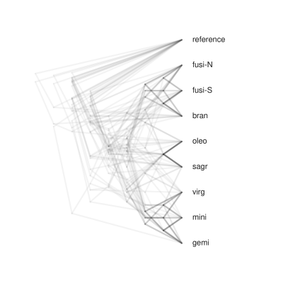
Draw cloud tree
Using toytree you can easily draw a cloud tree of overlapping gene trees to visualize discordance. These typically look much better if you root the trees, order tips by their consensus tree order, and do not use edge lengths. See below for an example, and see the toytree documentation.
[10]:
# filter to only windows with >50 SNPS (this could have been done in run)
trees = ts.tree_table[ts.tree_table.snps > 50].tree.tolist()

# load all trees into a multitree object
mtre = toytree.mtree(trees)

# root trees
mtre.treelist = [i.root("reference") for i in mtre.treelist]

# infer a consensus tree to get best tip order
ctre = mtre.get_consensus_tree()

# draw the first 12 trees in a grid
mtre.draw_cloud_tree(
    width=400,
    height=400,
    fixed_order=ctre.get_tip_labels(),
    use_edge_lengths=False,
);
Advanced: Modify the raxml command
In this analysis I entered multiple scaffolds to create windows across each scaffold. I also entered a smaller slide size than window size so that windows are partially overlapping. The raxml command string was modified to perform 10 full searches with no bootstraps.
[11]:
# select a scaffold idx, start, and end positions
ts = ipa.treeslider(
    name="chr1_w500K_s100K",
    data=data,
    workdir="analysis-treeslider",
    scaffold_idxs=[0, 1, 2],
    window_size=500000,
    slide_size=100000,
    minsnps=10,
    inference_method="raxml",
    inference_args={"m": "GTRCAT", "N": 10, "f": "d", 'x': None},
)
[12]:
# this is the tree inference command that will be used
ts.show_inference_command()
raxmlHPC-PTHREADS-SSE3 -f d -T 2 -m GTRCAT -n ... -w ... -s ... -p 54321 -N 10